Hardware:

HDD and SSD

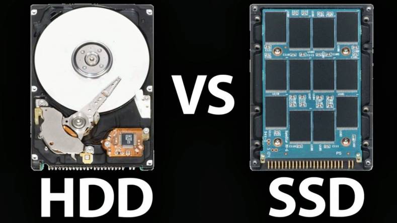
HDD:

HDDs are installed in most PCs and laptops. There are several aluminum plates inside the drive.
Reading and writing operations are performed due to rotation of the plates and the sensing head located at a few nanometers. The speed of the plates can be as high as 15,000 revolutions per minute which results in the common noise during operation.
These drives have become popular because they provide a lot of space (up to 4 TB on a single HDD), high reliability and stability during reading and writing operations.

Disadvantages of HDDs as compared to SSDs:

low speed of reading/writing operations
high power consumption
high noise level

Example:

Data storages

Backup systems

Large but not high loaded servers

High loaded web servers

SSD:

SSDs use memory chips and since they do not have any rotating elements, they are completely silent, consume less power and are smaller than HDDs. Reading and writing operations are performed faster in SSDs (files are opened, saved and deleted faster).

The relation of the data transfer rate to the size of the transmitted data block is defined by IOPS (Input/Output Operations Per Second). IOPS shows the number of blocks which can be read/ written per second. For reference, in HDDs this parameter is about 80-100 IOPS,while in SSDs it is more than 8,000 IOPS.

Example:
High-load projects
Content management system projects

RAID Levels

RAID is available in different schemes. The most commonly levels are RAID 0, 1, 5, 6, and 10. RAID 0, 1, and 5 work on both HDD and SSD media.

Raid 0: Striping

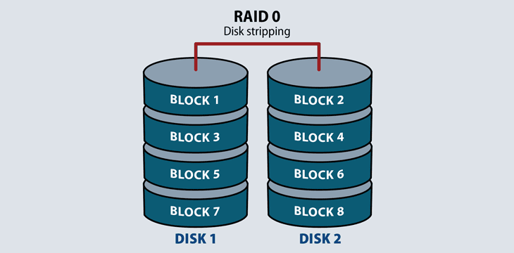
Requiring a minimum of two disks, RAID 0 splits files and stripes the data across two disks or more, treating the striped disks as a single partition. Because multiple hard drives are reading and writing parts of the same file at the same time, throughput is generally faster.

RAID 1: Mirroring

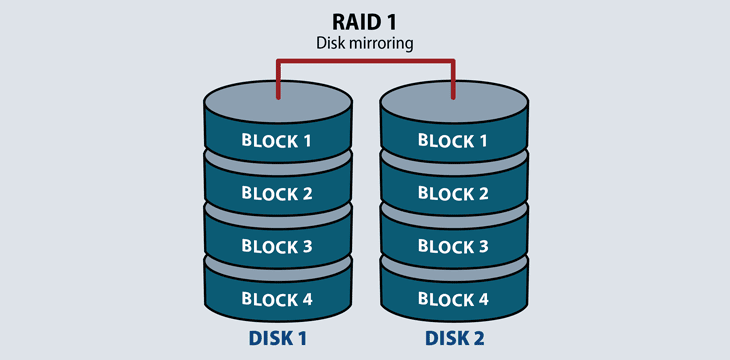
RAID 1 requires a minimum of two disks to work, and provides data redundancy and failover. It reads and writes the exact same data to each disk. Should a mirrored disk fail, the file exists in its entirety on the functioning disk. Once IT replaces the failed desk, the RAID system will automatically mirror back to the replacement drive. RAID 1 also increases read performance.

Raid 5: Striping with Parity

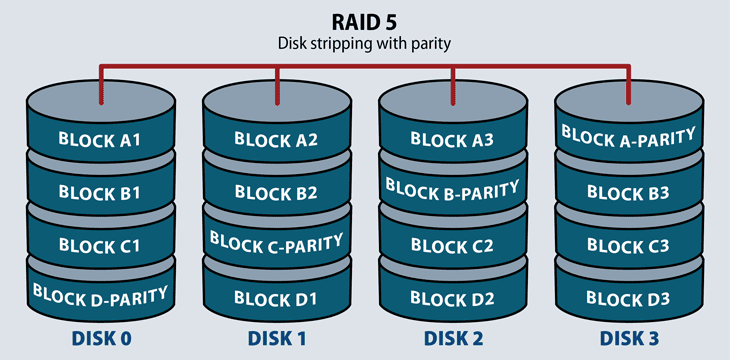
This RAID level distributes striping and parity at a block level. Parity is raw binary data. The RAID system calculates its values to create a parity block, which the system uses to recover striped data from a failed drive. Most RAID systems with parity functions store parity blocks on the disks in the array.
This level increases write performance since all drives in the array simultaneously serve write requests. However, overall disk performance can suffer from write amplification, since even minor changes to the stripes require multiple steps and recalculations.

RAID 6: Striping with double parity

RAID 6 offers higher redundancy than 5 and increased read performance. It can suffer from the same server performance overhead with intensive write operations. This performance hit depends on the RAID system architecture: hardware or software, if it’s located in firmware, and if the system includes processing software for high-performance parity calculations.

RAID 10: Striping and Mirroring

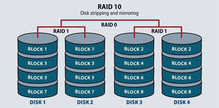
RAID 10 requires a minimum of four disks in the array. It stripes across disks for higher performance, and mirrors for redundancy. In a four-drive array, the system stripes data to two of the disks. The remaining two disks mirror the striped disks, each one storing half of the data.
This RAID level serves environments that require both high data security and high performance, such as high transactional databases that store sensitive information. It is the most expensive of the RAID levels with lower usable capacity and high system costs.

Software:

PostgreSQL Server Parameter Tuning:

1. max_connections = - Depending on your application it may be better to deny the connection entirely rather than degrade the performance of all of the other children.

2. shared_buffers = — Editing this option is the simplest way to improve the performance of your database server. General wisdom says that this should be set to roughly 25% of available RAM on the system.

3. effective_cache_size = — The larger the value increases the likely hood of using an index. Often this is more than 50% of the total system memory.

4. work_mem = — This option is used to control the amount of memory using in sort operations and hash tables. This option was previously called sort_mem in older versions of PostgreSQL.

5. max_fsm_pages = — This option helps to control the free space map. When something is deleted from a table it isn't removed from the disk immediately, it is simply marked as "free" in the free space map. The space can then be reused for any new INSERTs that you do on the table. If your setup has a high rate of DELETEs and INSERTs it may be necessary increase this value to avoid table bloat.

6. fsync = — This option determines if all your WAL pages are fsync()'ed to disk before a transactions is committed. Having this on is safer, but can reduce write performance. If fsync is not enabled there is the chance of unrecoverable data corruption.
Turn this off at your own risk.

7. commit_delay = and commit_siblings = — These options are used in concert to help improve performance by writing out multiple transactions that are committing at once. If there are commit_siblings number of backends active at the instant your transaction is committing then the server waiting commit_delay microseconds to try and commit multiple transactions at once.

8. random_page_cost = — random_page_cost controls the way PostgreSQL views non-sequential disk reads. A higher value makes it more likely that a sequential scan will be used over an index scan indicating that your server has very fast disks.

9. wal_buffers = - PostgreSQL writes its WAL (write ahead log) record into the buffers and then these buffers are flushed to disk. The default size of the buffer, defined by wal_buffers, is 16MB, but if you have a lot of concurrent connections then a higher value can give better performance.

10. maintenance_work_mem = - maintenance_work_mem is a memory setting used for maintenance tasks. The default value is 64MB. Setting a large value helps in tasks like VACUUM, RESTORE, CREATE INDEX, ADD FOREIGN KEY and ALTER TABLE.

11. synchronous_commit - This is used to enforce that commit will wait for WAL to be written on disk before returning a success status to the client. This is a trade-off between performance and reliability. If your application is designed such that performance is more important than the reliability, then turn off synchronous_commit.

12. checkpoint_timeout, checkpoint_completion_target - This whole process involves expensive disk read/write operations. The checkpoint_timeout parameter is used to set time between WAL checkpoints. Setting this too low decreases crash recovery time, as more data is written to disk, but it hurts performance too since every checkpoint ends up consuming valuable system resources.

The checkpoint_completion_target is the fraction of time between checkpoints for checkpoint completion. A high frequency of checkpoints can impact performance. For smooth checkpointing, checkpoint_timeout must be a low value. Otherwise the OS will accumulate all the dirty pages until the ratio is met and then go for a big flush.

13. max_parallel_workers_per_gather - parallel query is a method used to increase the execution speed of sql queries by creating multiple query process that divide the workload of a sql statement and executing it in parallel a at the same time.

Tips:

tables can split multiple tables
  example for 25 columns on one table split the table for 5column per tables.

Step 1: How To identified the Performance Issue ongoing for os level or PostgreSQL Server Level
  Use: top command
  top process for postgresql note pid(process id)

Step 5:Business hours only vacuum and analyze or non-business hours use vacuum full and analyze commands

Step 6:explain analyze the particular query
Example:
postgres=# explain analyze SELECT * FROM tenk1 t1, tenk2 t2 WHERE t1.unique1 < 100 AND t1.unique2 = t2.unique2 ORDER BY t1.fivethous;
                                                                 QUERY PLAN
--------------------------------------------------------------------------------------------------------------------------------------------
Sort (cost=717.34..717.59 rows=101 width=488) (actual time=7.761..7.774 rows=100 loops=1)
   Sort Key: t1.fivethous
   Sort Method: quicksort Memory: 77kB
   -> Hash Join (cost=230.47..713.98 rows=101 width=488) (actual time=0.711..7.427 rows=100 loops=1)
         Hash Cond: (t2.unique2 = t1.unique2)
         -> Seq Scan on tenk2 t2 (cost=0.00..445.00 rows=10000 width=244) (actual time=0.007..2.583 rows=10000 loops=1)
         -> Hash (cost=229.20..229.20 rows=101 width=244) (actual time=0.659..0.659 rows=100 loops=1)
               Buckets: 1024 Batches: 1 Memory Usage: 28kB
               -> Bitmap Heap Scan on tenk1 t1 (cost=5.07..229.20 rows=101 width=244) (actual time=0.080..0.526 rows=100 loops=1)
                     Recheck Cond: (unique1 < 100)
                     -> Bitmap Index Scan on tenk1_unique1 (cost=0.00..5.04 rows=101 width=0) (actual time=0.049..0.049 rows=100 loops=1)
                           Index Cond: (unique1 < 100)
Planning time: 0.194 ms
Execution time: 8.008 ms

scanning methods:

Sequential Scan:
Sequential Scan in PostgreSQL scans the entire table to choose the desired rows. This is the least effective scanning method because it browses through the whole table as stored on disk. The optimizer may decide to perform a sequential scan if the condition column in the query does not have an index or if the optimizer anticipates that the condition will be met by most of the rows in the table.

Index Scan:
The Index Scan traverses the B-tree of an index and looks for matching entries in the B-tree leaf nodes. It then fetches the data from the table. The Index Scan method is considered for use when there is a suitable index and the optimizer predicts to return relatively few rows of the table.

Index Only Scan:
The Index Only Scan algorithm has been introduced in PostgreSQL 9.2. The advantage of this method is that it avoids the costly table access when the database can find the columns in the index itself.

Bitmap Scan:

Bitmap scan is a mix of Index Scan and Sequential Scan. It tries to solve the disadvantage of Index scan but still keeps its full advantage. As discussed above for each data found in the index data structure, it needs to find corresponding data in heap page.
So alternatively it needs to fetch index page once and then followed by heap page, which causes a lot of random I/O. So bitmap scan method leverage the benefit of index scan without random I/O.

This works in two levels as below:

ostgres=# explain SELECT * FROM demotable WHERE num < 210;

                                  QUERY PLAN

-----------------------------------------------------------------------------

Bitmap Heap Scan on demotable (cost=5883.50..14035.53 rows=213042 width=15)

   Recheck Cond: (num < '210'::numeric)

   -> Bitmap Index Scan on demoidx (cost=0.00..5830.24 rows=213042 width=0)

      Index Cond: (num < '210'::numeric)

(4 rows)

Bitmap Index Scan:
First it fetches all index data from the index data structure and creates a bit map of all TID. For simple understanding, you can consider this bitmap contains a hash of all pages (hashed based on page no) and
each page entry contains an array of all offset within that page.

Bitmap Heap Scan:
As the name implies, it reads through bitmap of pages and then scans data from heap corresponding
to stored page and offset. At the end, it checks for visibility and predicate etc and returns the tuple based on the outcome of all these checks.

Join Methods:

Nested Loop:
There are two main versions of the Nested Loop method:

Nested Loop With Inner Sequential Scan. For each element from the first table it checks every row of the second table using the Sequential Scan method. If the join condition is fulfilled, the row is returned. The method can be very costly and is most often used for small tables.

The second version, Nested Loop With Inner Index Scan, uses an index for the second table instead of the Sequential Scan.

Hash Join:
The right relation is first scanned and loaded into a hash table, using its join attributes as hash keys. Next the left relation is scanned and the appropriate values of every row found are used as hash keys to locate the matching rows in the table.
The Hash Join algorithm starts by preparing a hash table of the smaller table on the join key. Each row is stored in the hash table at the location specified by a deterministic hash function. Next, the larger table is scanned, probing the hash table to find the rows which meet the join condition.

Merge Join:
The Merge Join is similar to the Merge Sort algorithm. Before the tables are joined, they are both sorted by the join attribute. The tables are then scanned in parallel to find matching values. Each row is scanned once provided that there are no duplicates in the left table.
This method is preferred for large tables.

Step 7:Last Right and top arrow is first Scan so any seq scan change index scan
Example emp is sequence scan ongoing so your are create index emp table id column

How to change index scan
postgres=# set enable_indexscan TO on; //not going index scan after
SET
postgres=# set enable_seqscan TO off;
SET

Example:
postgres=# explain analyze select *from emp where id=100;
                                                     QUERY PLAN
---------------------------------------------------------------------------------------------------------------------
Seq Scan on emp (cost=10000000000.00..10000835070.51 rows=3 width=13) (actual time=0.040..2398.305 rows=3 loops=1)
   Filter: (id = 100)
   Rows Removed by Filter: 14999940
Planning Time: 0.089 ms
Execution Time: 2398.342 ms
(5 rows)

postgres=# create index in_emp_id ON emp(id);
CREATE INDEX
postgres=# explain analyze select *from emp where id=100;
QUERY PLAN
----------------------------------------------------------------------------------------------------------------
Index Scan using in_emp_id on emp (cost=0.43..8.08 rows=3 width=13) (actual time=8.559..8.571 rows=3 loops=1)
Index Cond: (id = 100)
Planning Time: 25.795 ms
Execution Time: 8.621 ms
(4 rows)

postgres=# set random_page_cost TO 1;
SET
postgres=# explain analyze select *from emp where id=100;
QUERY PLAN
----------------------------------------------------------------------------------------------------------------
Index Scan using in_emp_id on emp (cost=0.43..4.30 rows=3 width=13) (actual time=0.031..0.037 rows=3 loops=1)
Index Cond: (id = 100)
Planning Time: 0.106 ms
Execution Time: 0.064 ms
(4 rows)

postgres=# set cpu_tuple_cost TO 0.001;
SET
postgres=# explain analyze select *from emp where id=100;
QUERY PLAN
----------------------------------------------------------------------------------------------------------------
Index Scan using in_emp_id on emp (cost=0.43..4.24 rows=3 width=13) (actual time=0.031..0.037 rows=3 loops=1)
Index Cond: (id = 100)
Planning Time: 0.105 ms
Execution Time: 0.062 ms
(4 rows)

postgres=# select name from pg_settings where name like 'enable%';
name
--------------------------------
enable_bitmapscan
enable_gathermerge
enable_hashagg
enable_hashjoin
enable_indexonlyscan
enable_indexscan
enable_material
enable_mergejoin
enable_nestloop
enable_parallel_append
enable_parallel_hash
enable_partition_pruning
enable_partitionwise_aggregate
enable_partitionwise_join
enable_seqscan
enable_sort
enable_tidscan
(17 rows)

product=# select name from pg_settings where name like '%cost%' and name not like '%vacuum%';
name
-------------------------
cpu_index_tuple_cost
cpu_operator_cost
cpu_tuple_cost
jit_above_cost
jit_inline_above_cost
jit_optimize_above_cost
parallel_setup_cost
parallel_tuple_cost
random_page_cost
seq_page_cost
(10 rows)

Step 8: Reduce the random_page_cost and cpu_tuple_cost

product=# SET max_parallel_workers_per_gather TO default;
SET
product=# show max_parallel_workers_per_gather;
max_parallel_workers_per_gather
---------------------------------
2
(1 row)
=====================================================================================
Size Worker
<8MB 0
<24MB 1
<72MB 2
<216MB 3
<648MB 4
<1944MB 5
<5822MB 6

=================================================
hint plan:

PostgreSQL uses cost based optimizer, which utilizes data statistics, not static rules. The planner (optimizer) esitimates costs of each possible execution plans for a SQL statement then the execution plan with the lowest cost finally be executed. The planner does its best to select the best best execution plan, but not perfect, since it doesn't count some properties of the data, for example, correlation between columns.
pg_hint_plan makes it possible to tweak execution plans using so-called "hints", which are simple descriptions in the SQL comment of special form.

Install Hint plan:

# tar xzvf pg_hint_plan-1.x.x.tar.gz
# cd pg_hint_plan-1.x.x
# make
# make install

Loding pg_hint_plan:
postgres=# LOAD 'pg_hint_plan';
LOAD

Exaple:
postgres=# /*+
postgres*#    HashJoin(a b)
postgres*#    SeqScan(a)
postgres*# */
postgres-# EXPLAIN SELECT *
postgres-#    FROM pgbench_branches b
postgres-#    JOIN pgbench_accounts a ON b.bid = a.bid
postgres-#   ORDER BY a.aid;
                                      QUERY PLAN
---------------------------------------------------------------------------------------
Sort (cost=31465.84..31715.84 rows=100000 width=197)
   Sort Key: a.aid
   -> Hash Join (cost=1.02..4016.02 rows=100000 width=197)
         Hash Cond: (a.bid = b.bid)
         -> Seq Scan on pgbench_accounts a (cost=0.00..2640.00 rows=100000 width=97)
         -> Hash (cost=1.01..1.01 rows=1 width=100)
               -> Seq Scan on pgbench_branches b (cost=0.00..1.01 rows=1 width=100)
(7 rows)

Scan method hints:

Example:
postgres=# /*+
postgres*# SeqScan(t1)
postgres*# IndexScan(t2 t2_pkey)
postgres*# */
postgres-# SELECT * FROM table1 t1 JOIN table table2 t2 ON (t1.key = t2.key);

Join method hints:

Example:
postgres=# /*+
postgres*#     NestLoop(t1 t2)
postgres*#     MergeJoin(t1 t2 t3)
postgres*#     Leading(t1 t2 t3)
postgres*# */
postgres-# SELECT * FROM table1 t1
postgres-#     JOIN table table2 t2 ON (t1.key = t2.key)
postgres-#     JOIN table table3 t3 ON (t2.key = t3.key);

Joining order hints:

Example:
postgres=# /*+ Leading((t1 (t2 t3))) */ SELECT...

Row number correction hints:
Example:
postgres=# /*+ Rows(a b #10) */ SELECT... ; Sets rows of join result to 10
postgres=# /*+ Rows(a b +10) */ SELECT... ; Increments row number by 10
postgres=# /*+ Rows(a b -10) */ SELECT... ; Subtracts 10 from the row number.
postgres=# /*+ Rows(a b *10) */ SELECT... ; Makes the number 10 times larger.

GUC temporarily setting:

Example:
postgres=# /*+
postgres*# Set(random_page_cost 2.0)
postgres*# */
postgres-# SELECT * FROM table1 t1 WHERE key = 'value';

Search This Blog

DBA Master

PostgreSQL Performance Tuning

Hardware:

HDD and SSD

RAID Levels

Software:

PostgreSQL Server Parameter Tuning:

=================================================
hint plan:

Comments

Post a Comment

PostgreSQL Performance Tuning

Hardware:

HDD and SSD

RAID Levels

Software:

PostgreSQL Server Parameter Tuning:

=================================================hint plan:

Comments

Post a Comment

=================================================
hint plan: